Fibermagic Tutorial¶

Fibermagic is an open-source software package for the analysis of photometry data. It is written in Python and operates on pandas and numpy dataframes.

Fiber Photometry is a novel technique to capture neural activity in-vivo with a subsecond temporal precision. Genetically encoded fluorescent sensors are expressed by either transfection with an (AAV)-virus or transgenic expression. Strenght of fluorescence is dependent on the concentration of the neurotransmitter the sensor detects. Using an optic glas fiber, it is possible to image neural dynamics and transmitter release.

FP image

graphik source: https://en.wikipedia.org/wiki/Fiber_photometry

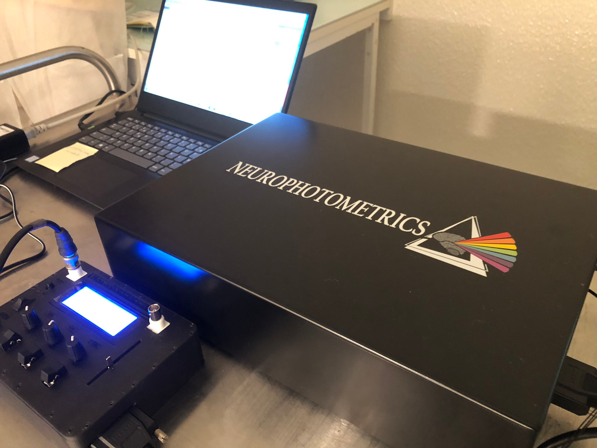
Fiber Photometry using Neurophotometrics devices¶

There are a bunch of different photometry systems out there like TDT systems, Neurophotometrics or open-hardware approaches. In this tutorial, we will use data from Neurophotometrics as an example.

NPM

Multiple Colors¶

With Neurophotometrics (NPM), it is possible to capture data from two fluorescent sensors simultaneously - if they emit light in different wave lengths. NPM can measure light of two different color spectra: Red and Green. Using this technology, it is possible, to e.g. express a green calcium sensor (e.g. GCaMP6f) and a red dopamine sensor (e.g. Rdlight1).

grafik source: https://www.researchgate.net/publication/264796291_Bright_and_fast_multi-colored_voltage_reporters_via_electrochromic_FRET/figures?lo=1

Multiple Mice¶

NPM can record data from multiple mice at once - delivered through a single path chord that splits into several small cables that can be attached individually to a single mouse.

The end of the patch chord projects to a photosensor which captures the light. Here’s how it looks like:

Multiple Mice

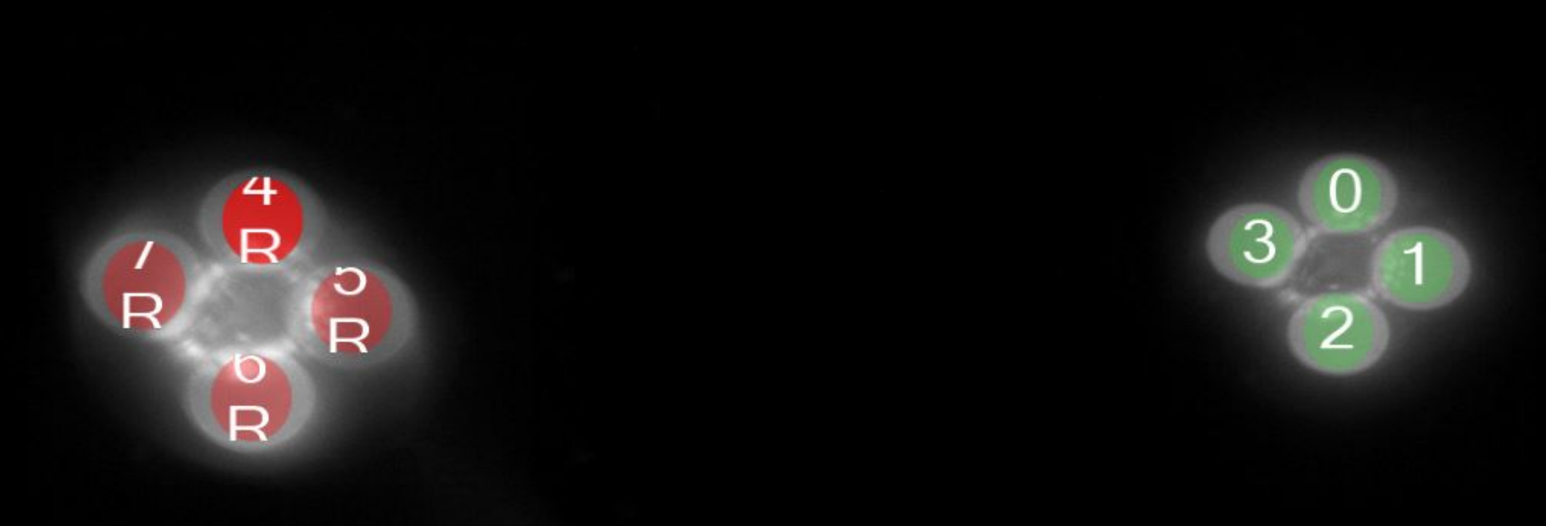
Before starting the recording, the researcher defines a region of interest for each cable and color. Then, NPM captures the light intensity for each region of interest seperately. All data streams are written into one single csv file per recording.

Investigating a single raw data file¶

Let’s have a look into an arbitrary recording file and try to understand the data.

[1]:

!pip install fibermagic
import pandas as pd
from fibermagic.utils.download_dataset import download
download('tutorial')

Requirement already satisfied: fibermagic in c:\users\georg\git\fibermagic (0.1.4)
Requirement already satisfied: numpy in c:\users\georg\anaconda3\envs\fibermagic\lib\site-packages (from fibermagic) (1.21.4)
Requirement already satisfied: pandas in c:\users\georg\anaconda3\envs\fibermagic\lib\site-packages (from fibermagic) (1.3.4)
Requirement already satisfied: matplotlib in c:\users\georg\anaconda3\envs\fibermagic\lib\site-packages (from fibermagic) (3.5.1)
Requirement already satisfied: scipy in c:\users\georg\anaconda3\envs\fibermagic\lib\site-packages (from fibermagic) (1.7.2)
Requirement already satisfied: scikit-learn in c:\users\georg\anaconda3\envs\fibermagic\lib\site-packages (from fibermagic) (1.0.1)
Requirement already satisfied: plotly in c:\users\georg\anaconda3\envs\fibermagic\lib\site-packages (from fibermagic) (5.4.0)
Requirement already satisfied: dash in c:\users\georg\anaconda3\envs\fibermagic\lib\site-packages (from fibermagic) (2.0.0)
Requirement already satisfied: Flask>=1.0.4 in c:\users\georg\anaconda3\envs\fibermagic\lib\site-packages (from dash->fibermagic) (2.0.2)
Requirement already satisfied: dash-table==5.0.0 in c:\users\georg\anaconda3\envs\fibermagic\lib\site-packages (from dash->fibermagic) (5.0.0)
Requirement already satisfied: dash-core-components==2.0.0 in c:\users\georg\anaconda3\envs\fibermagic\lib\site-packages (from dash->fibermagic) (2.0.0)
Requirement already satisfied: dash-html-components==2.0.0 in c:\users\georg\anaconda3\envs\fibermagic\lib\site-packages (from dash->fibermagic) (2.0.0)
Requirement already satisfied: flask-compress in c:\users\georg\anaconda3\envs\fibermagic\lib\site-packages (from dash->fibermagic) (1.10.1)
Requirement already satisfied: tenacity>=6.2.0 in c:\users\georg\anaconda3\envs\fibermagic\lib\site-packages (from plotly->fibermagic) (8.0.1)
Requirement already satisfied: six in c:\users\georg\anaconda3\envs\fibermagic\lib\site-packages (from plotly->fibermagic) (1.16.0)
Requirement already satisfied: packaging>=20.0 in c:\users\georg\anaconda3\envs\fibermagic\lib\site-packages (from matplotlib->fibermagic) (21.3)
Requirement already satisfied: pyparsing>=2.2.1 in c:\users\georg\anaconda3\envs\fibermagic\lib\site-packages (from matplotlib->fibermagic) (3.0.6)
Requirement already satisfied: pillow>=6.2.0 in c:\users\georg\anaconda3\envs\fibermagic\lib\site-packages (from matplotlib->fibermagic) (8.4.0)
Requirement already satisfied: fonttools>=4.22.0 in c:\users\georg\anaconda3\envs\fibermagic\lib\site-packages (from matplotlib->fibermagic) (4.28.2)
Requirement already satisfied: python-dateutil>=2.7 in c:\users\georg\anaconda3\envs\fibermagic\lib\site-packages (from matplotlib->fibermagic) (2.8.2)
Requirement already satisfied: cycler>=0.10 in c:\users\georg\anaconda3\envs\fibermagic\lib\site-packages (from matplotlib->fibermagic) (0.11.0)
Requirement already satisfied: kiwisolver>=1.0.1 in c:\users\georg\anaconda3\envs\fibermagic\lib\site-packages (from matplotlib->fibermagic) (1.3.2)
Requirement already satisfied: pytz>=2017.3 in c:\users\georg\anaconda3\envs\fibermagic\lib\site-packages (from pandas->fibermagic) (2021.3)
Requirement already satisfied: joblib>=0.11 in c:\users\georg\anaconda3\envs\fibermagic\lib\site-packages (from scikit-learn->fibermagic) (1.1.0)
Requirement already satisfied: threadpoolctl>=2.0.0 in c:\users\georg\anaconda3\envs\fibermagic\lib\site-packages (from scikit-learn->fibermagic) (3.0.0)
Requirement already satisfied: Werkzeug>=2.0 in c:\users\georg\anaconda3\envs\fibermagic\lib\site-packages (from Flask>=1.0.4->dash->fibermagic) (2.0.2)
Requirement already satisfied: click>=7.1.2 in c:\users\georg\anaconda3\envs\fibermagic\lib\site-packages (from Flask>=1.0.4->dash->fibermagic) (8.0.3)
Requirement already satisfied: itsdangerous>=2.0 in c:\users\georg\anaconda3\envs\fibermagic\lib\site-packages (from Flask>=1.0.4->dash->fibermagic) (2.0.1)
Requirement already satisfied: Jinja2>=3.0 in c:\users\georg\anaconda3\envs\fibermagic\lib\site-packages (from Flask>=1.0.4->dash->fibermagic) (3.0.3)
Requirement already satisfied: brotli in c:\users\georg\anaconda3\envs\fibermagic\lib\site-packages (from flask-compress->dash->fibermagic) (1.0.9)
Requirement already satisfied: colorama in c:\users\georg\anaconda3\envs\fibermagic\lib\site-packages (from click>=7.1.2->Flask>=1.0.4->dash->fibermagic) (0.4.4)
Requirement already satisfied: MarkupSafe>=2.0 in c:\users\georg\anaconda3\envs\fibermagic\lib\site-packages (from Jinja2>=3.0->Flask>=1.0.4->dash->fibermagic) (2.0.1)
Downloading started
Downloading Completed, Extracting...

[2]:

df = pd.read_csv('rawdata_demo.csv')
df.head(10)

[2]:

	FrameCounter	Timestamp	Flags	Region0R	Region1G	Region2R	Region3G	Region4R	Region5G	Region6R	Region7G
0	0	2955.990560	16	0.003922	0.003922	0.003922	0.003922	0.003922	0.003922	0.003922	0.003922
1	1	2956.003840	18	0.004341	0.007010	0.005176	0.008868	0.004264	0.006001	0.005350	0.007242
2	2	2956.017184	20	0.020586	0.350305	0.020055	0.310345	0.018077	0.380686	0.011893	0.189797
3	3	2956.030528	17	0.018014	0.015875	0.019811	0.017195	0.019681	0.024707	0.015898	0.014165
4	4	2956.043840	18	0.003923	0.004603	0.003935	0.007462	0.003922	0.004054	0.003966	0.004644
5	5	2956.057184	20	0.018542	0.344338	0.018014	0.304967	0.015870	0.374825	0.009874	0.185943
6	6	2956.070528	17	0.017936	0.015720	0.019849	0.017191	0.019787	0.024617	0.015881	0.014059
7	7	2956.083840	18	0.004350	0.007031	0.005192	0.008787	0.004257	0.005926	0.005291	0.007185
8	8	2956.097184	20	0.020549	0.345224	0.019962	0.305642	0.017845	0.375177	0.011721	0.187082
9	9	2956.110528	17	0.017933	0.015715	0.019841	0.017110	0.019732	0.024621	0.015832	0.014013

Each Region of Interest is represented as one column.

A simple frame counter and a timestamp indicate when a measurement happened.

The Flags column encodes different things: Which LED was on at the time of measurement, which input and/or output channel was on or off and whether the laser for optogenetic stimulation was on. NPM encodes all this information into a single number using a dual encoding.

Because the emission spectra of fluorescent proteins are partly overlapping, it is not possible to measure both, the red and green sensor, at the same time. Instead, only one LED is on at a time. That way, we get presice measurements.

rawdata

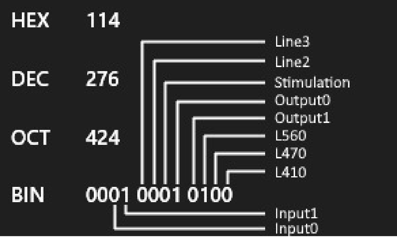
We can use fibermagic to decode which LEDs were on at what measurement from the Flags column.

[3]:

from fibermagic.IO.NeurophotometricsIO import extract_leds

[4]:

if 'Flags' in df.columns:  # legacy fix: Flags were renamed to LedState
    df = df.rename(columns={'Flags': 'LedState'})
df = extract_leds(df).dropna()
df.head(10)

[4]:

	FrameCounter	Timestamp	LedState	Region0R	Region1G	Region2R	Region3G	Region4R	Region5G	Region6R	Region7G	wave_len
1	1	2956.003840	18	0.004341	0.007010	0.005176	0.008868	0.004264	0.006001	0.005350	0.007242	470.0
2	2	2956.017184	20	0.020586	0.350305	0.020055	0.310345	0.018077	0.380686	0.011893	0.189797	560.0
3	3	2956.030528	17	0.018014	0.015875	0.019811	0.017195	0.019681	0.024707	0.015898	0.014165	410.0
4	4	2956.043840	18	0.003923	0.004603	0.003935	0.007462	0.003922	0.004054	0.003966	0.004644	470.0
5	5	2956.057184	20	0.018542	0.344338	0.018014	0.304967	0.015870	0.374825	0.009874	0.185943	560.0
6	6	2956.070528	17	0.017936	0.015720	0.019849	0.017191	0.019787	0.024617	0.015881	0.014059	410.0
7	7	2956.083840	18	0.004350	0.007031	0.005192	0.008787	0.004257	0.005926	0.005291	0.007185	470.0
8	8	2956.097184	20	0.020549	0.345224	0.019962	0.305642	0.017845	0.375177	0.011721	0.187082	560.0
9	9	2956.110528	17	0.017933	0.015715	0.019841	0.017110	0.019732	0.024621	0.015832	0.014013	410.0
10	10	2956.123840	18	0.004425	0.007011	0.005275	0.008732	0.004260	0.005959	0.005242	0.007178	470.0

Now, we have all we need to plot the full trace of a single sensor of one mouse and inspect the raw data values. In this recording, Rdlight1 and GCaMP6f were expressed. Rdlight1 is excited by the 560 nm LED and emits light in the red color spectrum. GCaMP6f is excited by the 470 nm LED and emits light in the green spectrum. Now, let’s spike into the raw data of Rdlight1 of a single mouse.

We use “plotly” for plotting here. Plotly is a plotting library for Python and other programming languages. It is interactive, which means we can zoom in and out and scroll through the data, which is exactly what we want to do at the moment.

[5]:

import plotly.express as px

[6]:

region0R_red = df[df.wave_len == 560][['FrameCounter', 'Region0R']]
px.line(region0R_red, x='FrameCounter', y='Region0R')

We can clearly see huge transients from dopamine activity in the raw data. Congratulations!

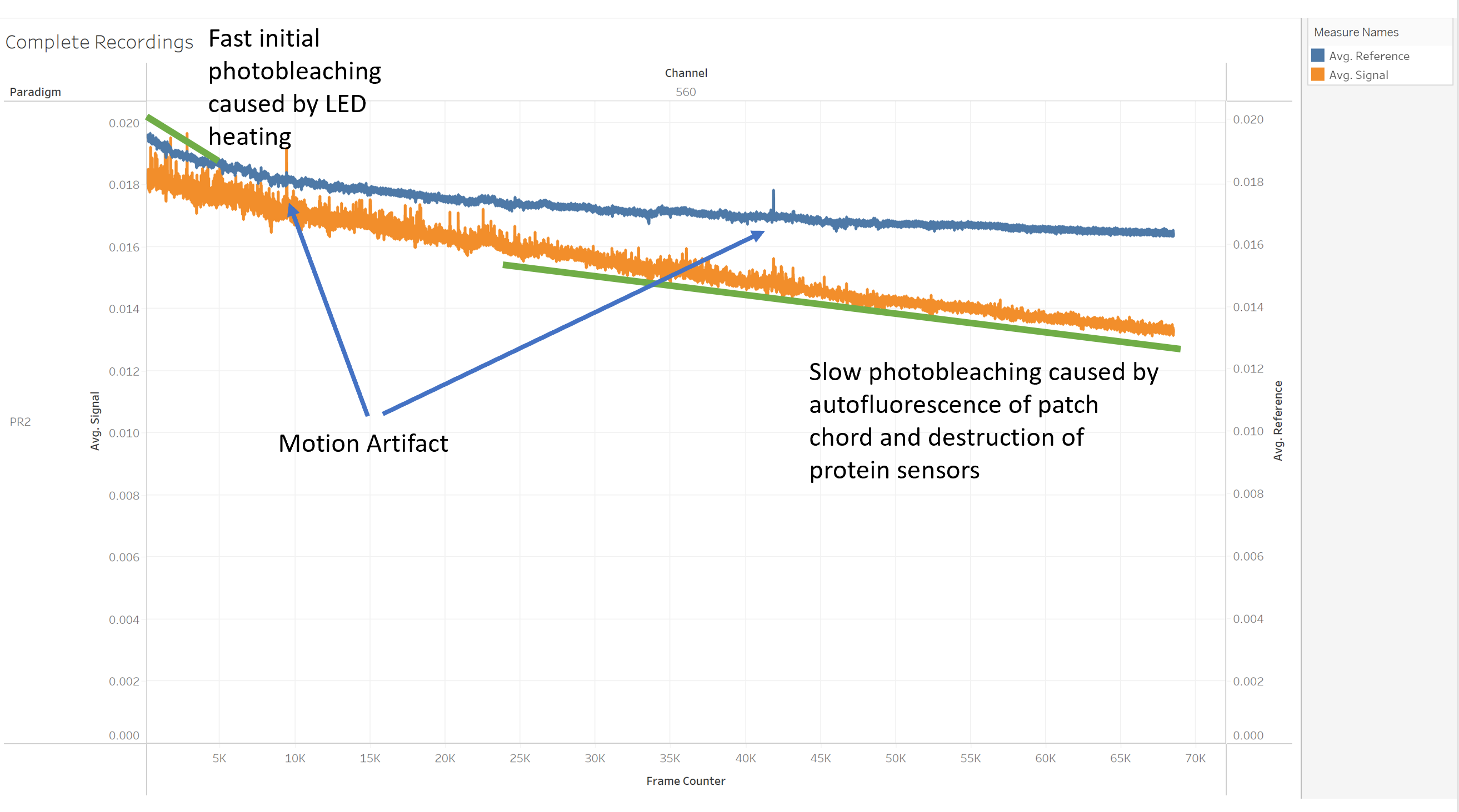
However, there are several issues with the data. Fiber Photometry is not measureing the difference between day and night. Changes in fluorescence are usually extremely small and very hard to measure. We basically measure light intensity with a super high precision. However, this means that the photometry system will also pick up every disturbance, even if very small.

Examples of unwanted noise are: * Photobleaching of the Patch Chord * Photobleaching caused by LED heating * Photobleaching caused by destroyment of sensors * Motion artifacts * Loose or poorly attached cables

photobleaching

Demodulation of Fiber Photometry Data¶

As we saw, the raw data is useless without further processing. There are a variety of different of different methods to remove photobleaching and motion artifacts, here are a few examples:

Correction of Photobleaching:¶

High-Pass Filtering: Photobleaching usually occurs at a very slow timescale. By applying a simple high-pass filter, e.g. a butterworth, it is possible to remove the gross artifacts of photobleaching, but it removes also slow changes in neurotransmitter concentration
Biexponential decay: Photobleaching can be estimated by a decreasing exponential function. However, as it happens on two different timescales (e.g. fast LED-heating-based photobleaching and slow patch chord photobleaching), we need a biexponential decay that can be regressed to the data and then subtracted.
airPLS: Adaptive iteratively reweighted penalized least squares. A more advanced method to remove artifacts. For more info, please see the paper: DOI: 10.1039/b922045c

Correction of Motion Artifacts:¶

Genetically encoded Neurotransmitter indicators have usually a useful attribute: If stimulated at around 410 nm (instead of e.g. 470 or 560), the excitation will be the same independent of the neurotransmitter concentration. Stimulating a this wave length is called recording an “isobestic”. The isobestic is usefull to correct motion artifacts.
If a transient is caused by neural activity, it should be detectable in the signal channel, but if it is caused by motion, it should be detectable in both, the isobestic and signal.
We can remove motion artifacts if we fit the isobestic to the signal and subtract.

Demodulate using airPLS¶

We can use fibermagic to calculate z-scores of dF/F using the airPLS algorithm. However, before we do that, we need to bring the dataframe into long-format.

[7]:

NPM_RED = 560
NPM_GREEN = 470
NPM_ISO = 410
# dirty hack to come around dropped frames until we find better solution -
# it makes about 0.16 s difference
df.FrameCounter = df.index // len(df.wave_len.unique())
df = df.set_index('FrameCounter')
regions = [column for column in df.columns if 'Region' in column]
dfs = list()
for region in regions:
    channel = NPM_GREEN if 'G' in region else NPM_RED
    sdf = pd.DataFrame(data={
        'Region': region,
        'Channel': channel,
        'Signal': df[region][df.wave_len == channel],
        'Reference': df[region][df.wave_len == NPM_ISO]
    }
    )
    dfs.append(sdf)
dfs = pd.concat(dfs).reset_index().set_index(['Region', 'Channel', 'FrameCounter'])
dfs

[7]:

			Signal	Reference
Region	Channel	FrameCounter
Region0R	560	0	0.020586	NaN
		1	0.018542	0.018014
		2	0.020549	0.017936
		3	0.020701	0.017933
		4	0.021635	0.018000
...	...	...	...	...
Region7G	470	68674	0.005743	0.010064
		68675	0.005734	0.010049
		68676	0.005767	0.010081
		68677	0.005793	0.010060
		68678	NaN	0.010077

549432 rows × 2 columns

[8]:

from fibermagic.core.demodulate import add_zdFF

dfs = add_zdFF(dfs, method='airPLS', remove=250)

[9]:

dfs

[9]:

		FrameCounter	Signal	Reference	zdFF (airPLS)
Region	Channel
Region0R	560	251	0.020384	0.017583	-1.751040
	560	252	0.020382	0.017586	-1.751065
	560	253	0.020450	0.017540	-1.715426
	560	254	0.020423	0.017533	-1.596002
	560	255	0.020440	0.017572	-1.544472
...	...	...	...	...	...
Region7G	470	68423	0.005653	0.010038	-1.173983
	470	68424	0.005743	0.010010	-0.189733
	470	68425	0.005760	0.010022	0.253415
	470	68426	0.005812	0.009984	0.270365
	470	68427	0.005806	0.009965	0.285169

545416 rows × 4 columns

[10]:

fig = px.line(dfs.reset_index(), x='FrameCounter', y='zdFF (airPLS)', facet_row='Region', height=1000)
fig.for_each_annotation(lambda a: a.update(text=a.text.split("=")[-1]))
fig

Analyzing and Synchronizing Behavioral Data¶

In almost all experiments, we want to collect behavioral data along with the neural data. We then want to correlate the mice’s behavior with our neural recording. For example, the mouse might perform a lever pressing task in an operand box. The operand box collects data about the time when the lever is pressed and when a food reward is delivered.

Let’s have a look into the log file produced by the operant box

[11]:

logs = pd.read_csv('operand_box.log')
logs

[11]:

	2021-10-15	12:46	1	186817	SI@0.0
0	2021-10-15	12:46	1	0	P0@0.0
1	2021-10-15	12:46	1	2634	RL@26.49
2	2021-10-15	12:47	1	7144	RL@71.49
3	2021-10-15	12:47	1	10001	SI@100.0
4	2021-10-15	12:47	1	13288	RL@132.8
...	...	...	...	...	...
711	2021-10-15	13:31	1	2675479	SI@26700.0
712	2021-10-15	13:31	1	2685501	SI@26800.0
713	2021-10-15	13:31	1	2695524	SI@26900.0
714	2021-10-15	13:31	1	2700001	ST@26944.68
715	2021-10-15	13:31	1	2700004	P1@26944.71

716 rows × 5 columns

As we see, the column “SI@0.0” records the type of event (e.g. left lever pressed; food delivered, etc…) and the time.

There are a variety of possibilities how to synchronize the logs with the FP data. In this case, an external generator generates a TTL pulse every 100 ms. The TTL pulse is captured by the operand box and logged as SI. The TTL pulse is also captured by the “input1” channel of NPM and saved in “input1.csv”.

Luckily, fibermagic offers functionality to synchronize both.

[12]:

from fibermagic.IO.NeurophotometricsIO import sync_from_TTL_gen
from pathlib import Path

logs = sync_from_TTL_gen(logs, Path('.'))
logs

[12]:

	Event	Timestamp
FrameCounter
133	P0	0.00
198	RL	26.49
311	RL	71.49
383	SI	100.00
464	RL	132.80
...	...	...
67026	SI	26700.00
67277	SI	26800.00
67527	SI	26900.00
67637	ST	26944.68
67637	P1	26944.71

716 rows × 2 columns

We see that the column ‘FrameCounter’ was added to the dataframe. Now we know exactly where in the photometry data an event happened.

Plot Perievents¶

With the synchronization done, we can finally extract a few seconds before and after each event and investigate if there is a common pattern. This is called calculating perievents.

[13]:

logs['Region'] = 'Region6R'
logs = logs.set_index('Region', append=True).swaplevel()
logs

[13]:

		Event	Timestamp
Region	FrameCounter
Region6R	133	P0	0.00
	198	RL	26.49
	311	RL	71.49
	383	SI	100.00
	464	RL	132.80
	...	...	...
	67026	SI	26700.00
	67277	SI	26800.00
	67527	SI	26900.00
	67637	ST	26944.68
	67637	P1	26944.71

716 rows × 2 columns

[14]:

from fibermagic.core.perievents import perievents

peri = perievents(dfs.set_index('FrameCounter', append=True), logs[logs.Event=='FD'], window=5, frequency=25)
peri

c:\users\georg\git\fibermagic\fibermagic\core\perievents.py:41: SettingWithCopyWarning:


A value is trying to be set on a copy of a slice from a DataFrame.
Try using .loc[row_indexer,col_indexer] = value instead

See the caveats in the documentation: https://pandas.pydata.org/pandas-docs/stable/user_guide/indexing.html#returning-a-view-versus-a-copy

C:\Users\Georg\anaconda3\envs\fibermagic\lib\site-packages\pandas\core\frame.py:3678: SettingWithCopyWarning:


A value is trying to be set on a copy of a slice from a DataFrame.
Try using .loc[row_indexer,col_indexer] = value instead

See the caveats in the documentation: https://pandas.pydata.org/pandas-docs/stable/user_guide/indexing.html#returning-a-view-versus-a-copy

c:\users\georg\git\fibermagic\fibermagic\core\perievents.py:58: SettingWithCopyWarning:


A value is trying to be set on a copy of a slice from a DataFrame.
Try using .loc[row_indexer,col_indexer] = value instead

See the caveats in the documentation: https://pandas.pydata.org/pandas-docs/stable/user_guide/indexing.html#returning-a-view-versus-a-copy

[14]:

					Signal	Reference	zdFF (airPLS)
Region	Channel	Event	Timestamp	Trial
Region6R	560	FD	-5.00	0	0.011402	0.014532	-0.778556
			-4.96	0	0.011420	0.014446	-0.895064
			-4.92	0	0.011426	0.014516	-1.030867
			-4.88	0	0.011398	0.014483	-1.056868
			-4.84	0	0.011424	0.014506	-1.284878
			...	...	...	...	...
			4.84	18	0.009506	0.012509	1.369639
			4.88	18	0.009463	0.012521	1.555787
			4.92	18	0.009525	0.012492	1.517118
			4.96	18	0.009431	0.012533	1.625856
			5.00	18	0.009499	0.012598	1.603165

4769 rows × 3 columns

[15]:

fig = px.scatter(peri.reset_index(), x='Timestamp', y='Trial', color='zdFF (airPLS)', range_color=(-5,5),
                 color_continuous_scale=['blue', 'grey', 'red'], height=250).update_yaxes(autorange="reversed")
for scatter in fig.data:
    scatter.marker.symbol = 'square'
fig.show()

How to analyze big projects¶

So far, we analyzed one single mouse, one single recording, one single channel. However, in practice, we usually record from 10-20 mice per experiment and have multiple long recordings. This adds up easily to several hundret files together with all the logs produced. It would be very time consuming and error-prone if a researcher would have to analyze every single file on its own.

Fortunately, fibermagic offers functionality to process a full project at once and fully automatically. In addition, fibermagic is very fast and can process full projects within seconds. Ultimately, you can use the same functions, no matter if you load a full project or a single file.

The only thing you have to do is to structure your project into a tree of directories with one category per level. For example, you may want to structure your project into experimental group (condition/control), experimental procedure (e.g. PR2, PR5, PR8, PR11) and recording (e.g. R1, R2, R3). You have to organize your recordings into subdirectories.

== condition
      =PR2
          =R1
               data.csv
               input1.csv
               regions_to_mouse.csv
               time.csv
               logs.csv
          =R2
          =R3
      =PR5
      =PR8
      =PR11
 = control

[ ]:

from fibermagic.IO.NeurophotometricsIO import read_project_logs, read_project_rawdata

download('fdrd2xadora_PR_Pilot')
help(read_project_rawdata)
help(read_project_logs)

Downloading started

[ ]:

project_path = Path(r'fdrd2xadora_PR_Pilot')
logs = read_project_logs(project_path,
                                 ['Paradigm'], ignore_dirs=['meta', 'processed'])
df = read_project_rawdata(project_path,
                          ['Paradigm'], 'FED3.csv', ignore_dirs=['meta', 'processed'])
df = add_zdFF(df, smooth_win=10, remove=200).set_index('FrameCounter', append=True)
peri = perievents(df, logs[logs.Event == 'FD'], 5, 25)

output_path = project_path / 'processed'

# uncomment if you like to save the output files
#df.to_csv(output_path / 'datastream.csv')
#logs.to_csv(output_path / 'logs.csv')
#peri.to_csv(output_path / 'perievents.csv')

[ ]:

peri = peri.reset_index()
fig = px.scatter(peri[peri.Channel==560], x='Timestamp', y='Trial', color='zdFF (airPLS)', facet_row='Paradigm', facet_col='Mouse',
          range_color=(-5,5), facet_row_spacing=0, facet_col_spacing=0, width=140*len(peri.Mouse.unique()),
                 color_continuous_scale=['blue', 'grey', 'red']).update_yaxes(autorange="reversed")
for scatter in fig.data:
    scatter.marker.symbol = 'square'
fig.for_each_annotation(lambda a: a.update(text=a.text.split("=")[-1]))
fig.update_xaxes(range = [peri.Timestamp.min(),peri.Timestamp.max()])
fig.update_xaxes(matches='x')
fig.show()

[ ]:

peri

[ ]: